Testing, Data types and Reading in data

Introduction

Session overview

This week we cover how we can classify variables in terms of the type of values they can take and their role in analysis. We consider the impact variable type has on the tests that we conduct. In RStudio, we learn to read in data files and to summarise and plot data. We also cover saving figures and laying out a report in word.

Artwork by Allison Horst

Learning Outcomes

By actively following the lecture and practical and carrying out the independent study the successful student will be able to:

• to able to explain what response and explanatory variables are, distinguish between data types and describe how these impact choice of test (MLO 1 and 2)
• demonstrate the process of hypothesis testing with an example and evaluate potential inferences (MLO 1 and 2)
• read in data in to RStudio, create simple summaries and plots using manual pages where necessary (MLO 3)
• create neat reports in Word which include text and figures (MLO 4)

Philosophy

Workshops are not a test. It is expected that you often don’t know how to start, make a lot of mistakes and need help. Do not be put off and don’t let what you can not do interfere with what you can do. You will benefit from collaborating with others and/or discussing your results.

The lectures and the workshops are closely integrated and it is expected that you are familar with the lecture content before the workshop. You need not understand every detail as the workshop should build and consolidate your understanding. You may wish to refer to the slides as you work through the workshop schedule.

Slides

Tests, Data types and Reading in data: pdf (recommended) / pptx

Your responses from TurningPoint.

Getting started

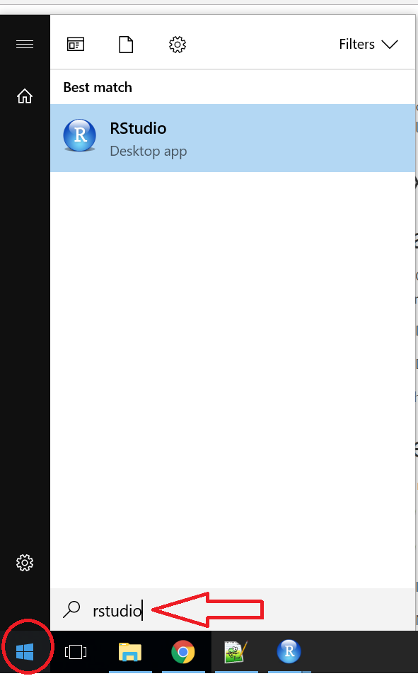
Start RStudio from the Start menu.

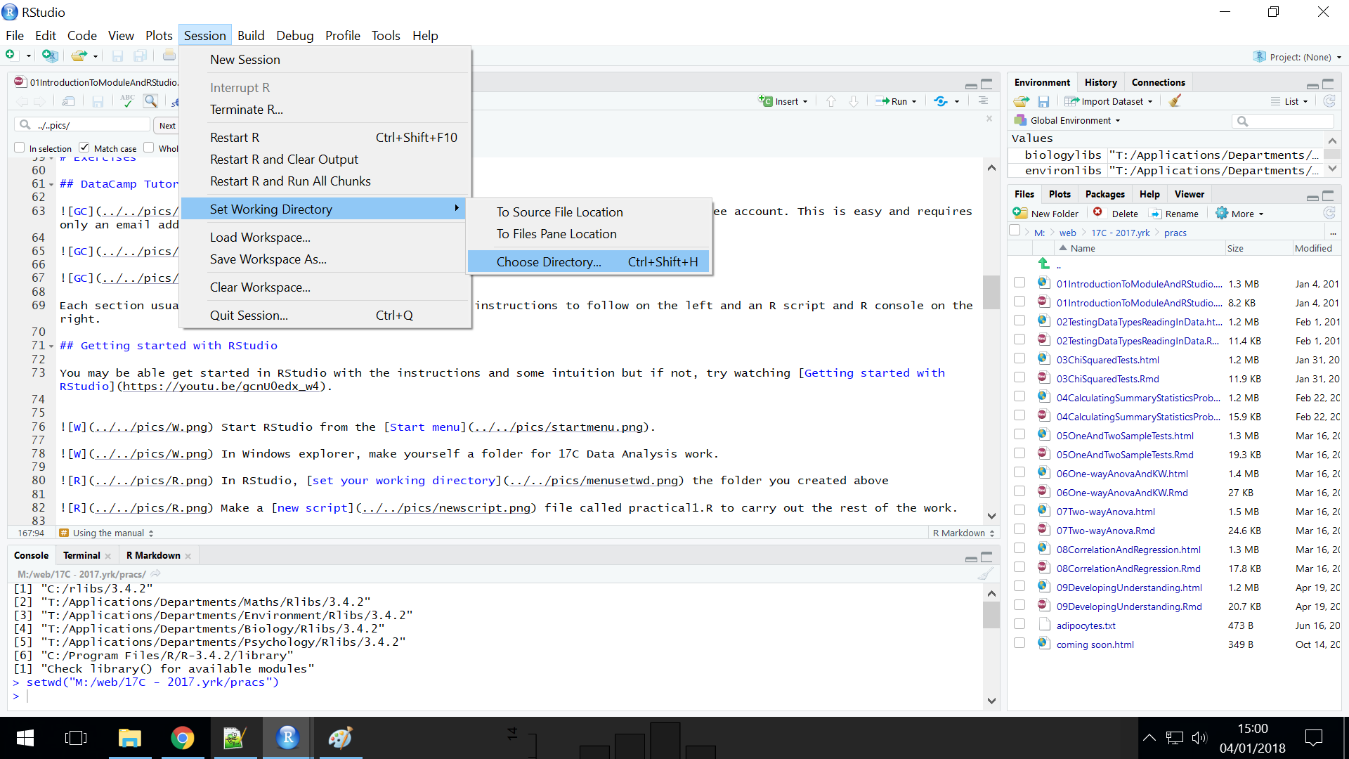
In RStudio, set your working directory to the folder you created last week for your 17C Data Analysis work.

Make a new script file called practical2.R to carry out the rest of the work.

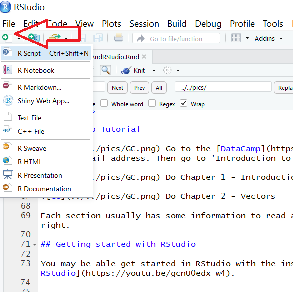
Exercises

Import Data

The data in pigeon.txt are 40 measurements of interorbital width (in mm) in a sample of domestic pigeons measured to the nearest 0.1mm

Save a copy (right click and Save) to your working directory

Read the data in to R by using the read.table() command:

pigeon <- read.table("pigeon.txt")

You should find an object called pigeon can be seen in the Environment window. If you click on that object a view of the data appears in the same window as the script.

Use str() to see what data structure is created

Change the variable name using names()

names(pigeon)[1] <- "interorbital"

#and look again with str
str(pigeon)

## 'data.frame':    40 obs. of  1 variable:
##  $ interorbital: num  12.2 12.9 11.8 11.9 11.6 11.1 12.3 12.2 11.8 11.8 ...

Exploring single group data

Values can be extract by indexing - giving the row number (r) and column number (c) of the element you want: pigeon[r, c]

The column is referred to using either

1. the index pigeon[,1] (note pigeon[1] will also work because R assumes you mean the column if you give only one index for a dataframe)

2. or the dollar notation pigeon$interorbital.

Can you extract the 14th value in the column?

We can use the ‘base’ plotting system (as opposed to the ggplot plotting system) to make a histogram with:

hist(pigeon$interorbital)

Can you create this histogram by reading the manual page for hist()

Note: the x axis goes from 8 to 14 which is given by c(8,14) and to lose text you can set the appropriate argument to NULL.

It’s useful to learn to ggplot way to do a histogram as it is far more more useful when we do more complex figures. ggplot2 is one of the tidyverse packages.

Do a ggplot() histogram

# library statement is only needed once per session
library(tidyverse)

ggplot(data = pigeon, aes(x = interorbital)) +
  geom_histogram()

We can improve it by changes the number of bins

ggplot(data = pigeon, aes(x = interorbital)) +
  geom_histogram(bins = 10, colour = "black")

R provides many functions to allow you to make calculations on your data.

Find out which functions will calculate the mean, standard deviation and the number of cases, i.e., the length of the vector. Google or make intelligent guesses and verfiy with the manual.

Import Data 2

Now you will practice with ‘paths’ and ‘relative paths’. These are a threshold concept in computing.

The data in pigeon2.txt are similar data of interorbital distances in two columns rather than just one. They are from two different populations, A and B.

Make a folder in your working directory called ‘data’

Save a copy of pigeon2.txt to the ‘data’ folder

To read the data in to R you need to use the relative path to the file in the read.table() command:

data2 <- read.table("data/pigeon2.txt", header = TRUE)

The data/ part is the ‘relative path’ to the file. It says where the file is relative to your working directory: pigeon2.txt is inside a folder (directory) called ‘data’ which is in your working directory. header = TRUE tells R that first row of the data file contains the column names.

look at the structure of the dataframe data2 using str()

You can see that R has used the first value in each column as the variable name.

Find the mean for each population. Remember, to refer to a single column of the data we need to use the dollar notation

Tidy format

Instead of having a population in each column, we very often have, and want, data organised so the measurements are all in one column and a second column gives the group. This format is described as ‘tidy’ (Wickham 2014): it has a variable in each column and only one observation (case) per row.

We can put this data in such a format with the gather() function from the tidyverse:

To use gather you need to give a key which will become the name of the variable indicating which column (group) the value came from and a value which will become the name of the measurements (responses). Examine the structure

# library statement is only needed once per session
data3 <- gather(data = data2, key = population, value = distance)
str(data3)

## 'data.frame':    80 obs. of  2 variables:
##  $ population: chr  "A" "A" "A" "A" ...
##  $ distance  : num  12.4 11.2 11.6 12.3 11.8 10.7 11.3 11.6 12.3 10.5 ...

How do we find the mean for each group now? If we use mean(data3$distance) we will get the mean of the whole column, not the means for each population. We can use ‘selection’ to apply a function only where a particular condition is met. For example:

mean(data3$distance[data3$population == "A"])

## [1] 11.24

This selects the rows in column $distance where the value in column $population is equal to A. == means ‘is it equal to?’ rather than ‘make it equal to’ given by =

Find the mean for population B using data3

Since data are so often organised in this format (one column for the measure with additional columns giving the groups), R has easier ways to apply a function to each group. We can apply the mean function to the $distance column separately for each population using a combination of two tidyverse functions: group_by() and summarise() and the ‘pipe’ (%>%)

data3 %>% 
  group_by(population) %>% 
  summarise(mean(distance))

## # A tibble: 2 x 2
##   population `mean(distance)`
##   <chr>                 <dbl>
## 1 A                      11.2
## 2 B                      11.7

%>% is called the pipe. It is a special operator that is realtively new in R and makes code easier to read and write. Usually, when you want to give data to a function you pass it as an argument inside the brackets. The pipe allows you to have the data on the left, then a pipe then the function with and additional arguments. This especially useful when you want to apply one function after another. The independent study covers the pipe further.

As you can imagine, this is much more convenient than using selection when you have many different groups.

Find the number of cases and variance of each group using group_by() and summarise().

Word reports with figures

Now we will create a word document with some text and figures. I find the best way to include figures in a word document is to use a table with the borders turned off. This can make it easier to control the layout. This is what you are aiming for.

open a word document

add some text

insert a 2 x 2 table

merge the cells on the second row and add a figure legend

Create a histogram for each group, trying to match those illustrated.

Copy the figure using Export | Copy to the Clipboard

Paste in to a table cell in word

select the table and give it No borders

Independent study

You need to carry out this work before the next practical.

1. Understanding the pipe: %>%

The magrittr package (Bache and Wickham 2014) is part of the tidyverse and includes the pipe operater which can improve code readability by:

• structuring sequences of data operations left-to-right (as opposed to from the inside and out),
• minimizing the need for intermediates,
• making it easy to add steps anywhere in the sequence of operations.

For example, to apply a log-squareroot transformation you might use:

# generate some numbers
nums <- sample(1:100, size = 10, replace = FALSE)

# transformation either:
# a) nested functions
tnums <- log(sqrt(nums))
# b) intermediates
sqrtnums <- sqrt(nums)
tnums <- log(sqrtnums)

Nesting the functions means you have to read inside out and creating intermediates can be cluttered. The pipe allows you to avoid these by taking the output of one operation as the input of the next. The pipe has long been used by Unix operating systems (where the pipe operator is |). The R pipe operator is %>%, a short cut for which is ctrl-shift-M.

tnums <- nums %>% 
  sqrt() %>% 
  log()

This is short for

tnums <- nums %>% 
  sqrt(.) %>% 
  log(.)

Where . stands for the object being passed in. In most cases, you don’t need to include it but some functions require you to (for example when arguments are optional or there is ambiguity over which argument is meant).

A additional benefit of using the pipe is that solving problems step-by-step is made easier.

Also see Pipes in R Tutorial For Beginners - I think a better title for this article is “Pipes For Beginners to pipes but with intermediate R experience” because it goes further than you need to be able to understand the pipe ‘well enough’. However, it still contains some useful examples.

2. Myoglobin concentration

The myoglobin concentration of skeletal muscle of three species of seal in grams per kilogram of muscle was determined and the data are given in seal.txt. Each row represents an individual seal. The first column gives the myoglobin concentration and the second column indicates species. Can you write a single page word report which includes some summary statistics (for example the means and standard deviations) for each seal species and some figures?

3. Understanding Paths

Do make sure you understand what a path is What do we mean by paths?

4. Script example

This is an example of a well formatted analysis script appropriate for some of the work we have carried out in this practical. Read it, run it!

5. DataCamp Assignments

If you have not completed the other DataCamp assignments, you should still be able to access and complete them but they’ll be indicated as late.

The Code files

These contain answers and code even though they do not appear on the webpage itself.

Rmd file The Rmd file is the file I use to compile the practical. Rmd stands for R markdown allow R code and ordinary text to be inter weaved to produce well-formatted reports including webpages.

Plain script file This is plain script (.R) version of the practical

Script example

This is an example of a well formatted analysis script suitable for submitting with a research report

Script example

Objectives from previous sessions

Introduction to module and RStudio

• to explain why we need statistical tests and the logic of hypothesis testing (MLO 1)
• use the R command line as a calculator and to assign variables (MLO 3)
• create and use the basic data types in R (MLO 3)
• find their way around the RStudio windows (MLO 3)
• create, use and save a script file to run r commands (MLO 3)
• search and understand manual pages (MLO 3)

References

Bache, Stefan Milton, and Hadley Wickham. 2014. Magrittr: A Forward-Pipe Operator for R. https://CRAN.R-project.org/package=magrittr.

Wickham, Hadley. 2014. “Tidy Data.” Journal of Statistical Software, Articles 59 (10): 1–23.